Robot Perception in Harsh Industrial Environments: Three Sensor Swaps and What Finally Decided It
A robot's perception system is not finished the moment you buy the right sensor. This is the record of how DIDEN Robotics tested sensors across four rounds inside steel structures, and then built the evaluation criteria and the coordinate-frame pipeline that sit on top of them.

Blog
Before a robot can take a single step on an industrial site, it has to know what is in front of it. Inside a space walled with coated steel, though, bolting on a high-spec sensor does not get you that information. Light does not scatter off these surfaces. It bounces away in one direction, so the signal the sensor is waiting for never comes back. Add a welding arc firing at unpredictable intervals, and the sensor's job gets harder still.
These conditions are not unique to one industry. Anywhere large metal structures are assembled and welded, the surfaces reflect specularly, the spaces are tight, and the lighting is impossible to predict.
The difficult part is that no datasheet tells you which sensors hold up here and which ones fall apart. Published measurement ranges and accuracy figures assume ordinary surfaces. A highly reflective metal face combined with arc flash sits outside that assumption.
So DIDEN Robotics did not simply pick sensors from a catalog. The team measured each candidate in the actual working environment, ran the resulting data through the perception algorithms, and judged from there. The criterion was never the sensor's own spec. It was whether control still behaved correctly on top of the data that sensor produced.
The evaluation ran through four rounds.
Round | Approach | What it solved | Where it broke |
1 | Active stereo camera | Projected IR pattern gave correspondence on featureless surfaces | Depth map collapsed under welding arc |
2 | iToF depth camera | Robust to arc flash, much wider field of view | Dropouts on specular steel, narrow operating temperature range |
3 | SPAD receiver LiDAR | Cleared both arc flash and specular reflection, native 3D output | Heavy noise on highly reflective surfaces |
4 | APD receiver LiDAR (selected) | Signal held on reflective steel, accuracy improves with distance | Lower point density |
What separated the four rounds was how the receiving element handles strong light. Three principles guided the decision. First, we defined the evaluation method before running anything, using how far a point cloud deviates from the true plane as the metric and applying the same procedure across three working sites. Second, we chose accuracy over density. The LiDAR we rejected returned far more points in the same area, but those points were scattered above and below the actual plane. Third, we judged on algorithm behavior rather than sensor output, confirming the choice only after running the point cloud through registration against the structure's design drawings.
Settling on a sensor does not complete a perception system, though. Several sensors pointing in different directions still have to be bound into a single coordinate frame, and the resulting data still has to reach control in a form it can use.
Hardware Set the Starting Point
The first sensor we tried was a camera. Not because cameras offered the best perception, but because the mechanical design of DIDEN Spider, our quadruped robot at the time, left no room to mount a LiDAR. Cameras also cost considerably less, which made them the natural first attempt.
That constraint did not last. As the hardware design improved, mounting a LiDAR became possible, and at that point the candidate pool changed entirely. Perception followed the hardware's constraints, then the hardware changed in response to what perception needed. The same structure we had already worked through with actuators and learning repeated itself with sensors.
[Why quadrupeds, bipeds, and humanoids all walk the same way: co-designing actuators and learning]
Four Rounds of Field Testing
Each round solved a problem and surfaced a new one. What blocked us at one stage was genuinely resolved at the next, and in exchange something that had stayed hidden until then came into view.
Active Stereo: Broken by the Welding Arc
We started with an active stereo camera.
A stereo camera works the same way human binocular vision does. When two cameras sitting side by side capture the same point, its pixel position shifts slightly between the two images, and that shift is called disparity. Distance follows from disparity alone. Given the lens focal length and the baseline between the cameras, a larger disparity means closer and a smaller one means farther. The catch is that disparity shrinks in inverse proportion to distance, so the same pixel-level error translates into a much larger distance error the farther out you go.
The hard part is finding that same point. Align the two cameras horizontally and the corresponding point can only lie on the same horizontal line, which reduces the search to one dimension. From there, you pick the position whose surrounding texture matches best. The problem is a surface with no texture to begin with. On a white wall or a plain steel plate, there is nothing to tell you which pixel pairs with which. That is why an active stereo camera projects an infrared pattern to plant artificial texture. It worked. Under normal conditions, the depth map came back stable.
Welding is where it fell apart. The instant an arc fires, the amount of light reaching each camera swings differently across the scene. Once the premise behind matching breaks, the entire depth map goes with it. Our measurements showed exactly that: a depth map that was fine moments earlier collapsing during arc exposure. In an environment where welding runs continuously, this was not usable.
iToF: Survived the Arc, Lost the Steel
The next candidate was an iToF (Indirect Time-of-Flight) depth camera. Because it derives distance from the round trip of emitted light, texture no longer matters, and its field of view was far wider than the previous camera's.
iToF calculates distance from how far the phase of the returning light has shifted. It emits infrared modulated in a sine wave and measures indirectly through phase difference rather than timing the round trip directly. Because it can use standard CMOS (Complementary Metal-Oxide-Semiconductor) sensors, it produces dense, high-resolution range images at relatively low cost.
And it genuinely held up against arc flash. With no algorithmic step searching for correspondence between left and right images, there is no matching to break in the first place. Pixels hit directly by the arc lost their values, but the surrounding region stayed intact. The problem we hit with stereo was solved here.
Steel itself became the obstacle instead. For any ToF-family sensor to measure distance, the emitted light has to scatter off the surface so that some fraction returns to the receiver. Smooth metal behaves like a mirror, throwing light off at the angle of incidence and nowhere else. In this environment, iToF ran into three distinct failures.
Dropout: With almost no light returning toward the sensor, no distance value is generated at that point at all.
Saturation: When the steel faces the sensor head on, the opposite happens. Light returns so strongly that the receiving element cannot handle it, and values either spike or disappear the same way.
Multipath: When light reflected straight off an object mixes with light that arrived via a wall or floor, the phase measurement is corrupted. The inside of a metal structure combines strong reflection with tight spacing, which is exactly the condition that produces this error.
The consequences showed up in the perception algorithms. Performance in position estimation dropped sharply during motions that require fine terrain judgment, such as passing through an access hole between structural members. The issue was that usable data simply was not present where a decision had to be made, which meant every calculation built on it was affected.
Once we confirmed that surface condition alone changes the outcome, we designed the comparison tests around primer-coated steel. Applying primer shifts the surface toward diffuse reflection, specular return drops, and sensor data comes back normally.
There was another reason to move on. The operating temperature range of this iToF camera was narrow enough that it left little margin for a product going into the field. The hardware revision that made LiDAR mounting possible landed at the same time, so we moved to the next round.

What an iToF depth camera sees when it looks at coated steel. The black regions are where specular reflection prevented any distance value from being generated.

DIDEN Spider passing through an access hole between structural members. This is a stretch that demands fine terrain judgment, so missing data destabilizes position estimation immediately.
SPAD Receiver LiDAR: Noise Grows on Reflective Surfaces
The third round brought us to LiDAR. Because LiDAR actively emits a laser and measures distance directly from the return, ambient light and surface texture matter far less, and the output arrives as a set of 3D coordinates rather than a pixel image. It passed the arc flash test without issue.
The dToF (Direct Time-of-Flight) method that LiDAR uses captures the moment a photon arrives, which structurally eliminates the interpolation error that comes with estimating time from phase. Among the receiving elements that detect those photons, one has been commercialized comparatively recently and is now appearing in a growing number of products: SPAD (Single-Photon Avalanche Diode). Because it is designed to respond the instant a single photon lands, it picks up even very weak returns and reaches long distances, and it delivers higher point density as well.
The first LiDAR DIDEN Robotics selected belonged to this family. On paper, the conditions looked favorable: a full 360-degree horizontal field of view, a wide operating temperature range, and dense point output.
The measurements told a different story. Distance values taken against coated steel carried heavy noise, at a magnitude the robot could not work with when judging where to place a foot or how far a wall was. The result was consistent with what happens when a high-sensitivity receiver saturates under strong return light. The very sensitivity engineered to catch faint signals worked against it here.
The three sensors failed at different points, but the root cause was the same. None of them could handle the way coated steel sends light back.
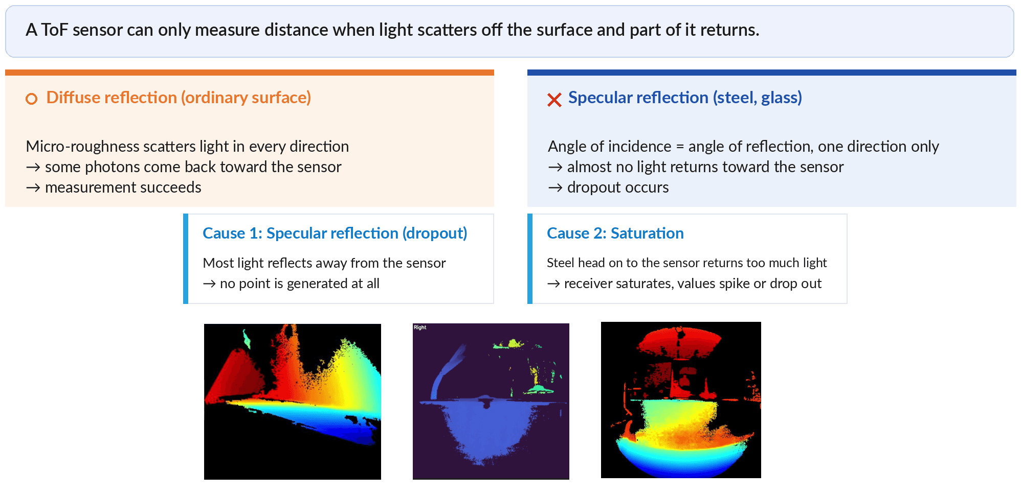
An ordinary surface scatters light in every direction, and some of it returns to the sensor. Smooth steel throws it off in a single direction. The three depth maps below show the result: values that are missing or wildly wrong.
The Receiver Architecture Made the Call
The sensor that survived was also a LiDAR. The difference was in the receiver.
SPAD receiver | APD receiver | |
Behavior | Fires on a single photon | Amplifies in proportion to incoming light |
Strengths | Weak returns, long range, low-reflectivity targets, high point density | Preserves intensity differences even under strong light |
On reflective metal | Prone to saturation from excess light | Signal holds |
SPAD is better at catching faint light, which makes it the stronger choice at long range and against low-reflectivity targets. In an environment like coated steel, where the intensity of returning light swings between extremes, the behavior of the APD (Avalanche Photodiode) is what decided the outcome.
We Built the Evaluation Method First
DIDEN Robotics measured both sensors directly and compared them. Comparing anything under equal conditions means first deciding what to measure and what counts as good, so the Perception team defined that standard and then carried out the measurements across three sites.
The metric was planar residual. Measure a flat wall and the points should land neatly on a single plane, but in practice they scatter slightly forward and back. That scatter is the planar residual, and the smaller it is, the more accurately the sensor read the surface. We measure it by cutting out only the flat steel region from the point cloud, computing the plane that best fits those points, and then measuring how far each point sits from it.
We chose this metric for two reasons. One is that it removes the need to know in advance exactly where the wall is. All you need is the fact that the steel is flat, which makes the test easy to repeat on site. The other is that the value connects directly to what the robot has to decide. A robot places its feet and holds its posture based on where the walls and floor are.
Testing ran at three real working sites enclosed by primer-coated steel. We combined mounting distance, mounting height, and viewing direction across wall and floor surfaces, including an extreme close-range condition of roughly 15 cm from the wall.
The results converged. Across all six combinations of site and surface, the APD receiver LiDAR produced the lower planar residual, and the ranking did not shift between indoor and outdoor settings.
The Two Sensors Moved in Opposite Directions
More telling than the averages was how each sensor behaved with distance. They moved in exactly opposite directions. The APD receiver LiDAR grew more accurate as distance increased, reaching its best around 0.9 m, while the SPAD receiver LiDAR degraded over the same span. At close range, around 0.3 m, the two were comparable, and under some conditions the SPAD unit was slightly better.
That difference maps onto the range the robot actually relies on. When the robot fixes its own position against walls and structural members, it works mostly in the 0.6-0.9 m band, which is precisely where the gap between the two sensors opened widest.
Viewing the point cloud as a cross-section makes the difference visible. The APD cloud converges into a thin band along the reference plane as distance grows, while the SPAD cloud either ripples along that plane or spreads thickly above and below it.
The extreme close range separated them as well. At roughly 15 cm, the SPAD receiver LiDAR showed a larger error at one site than it did elsewhere, and under other conditions we observed outliers that departed sharply from the reference plane. Even when averages look similar, a single outlier is the more dangerous failure for a robot deciding where to put its foot.
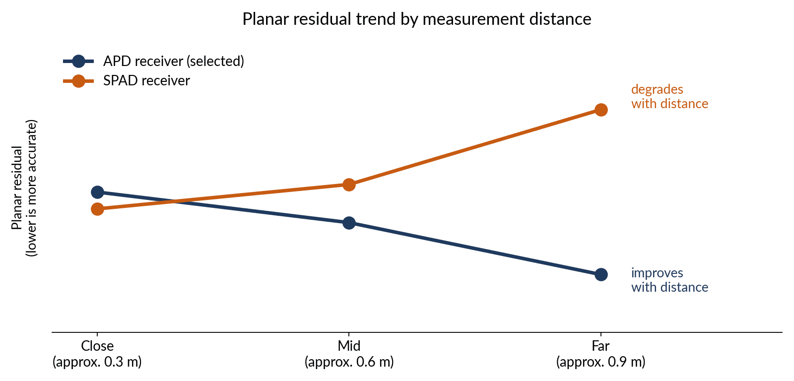
As distance grows, one sensor's error falls and the other's rises. The band where the robot fixes its position is where the gap is widest.
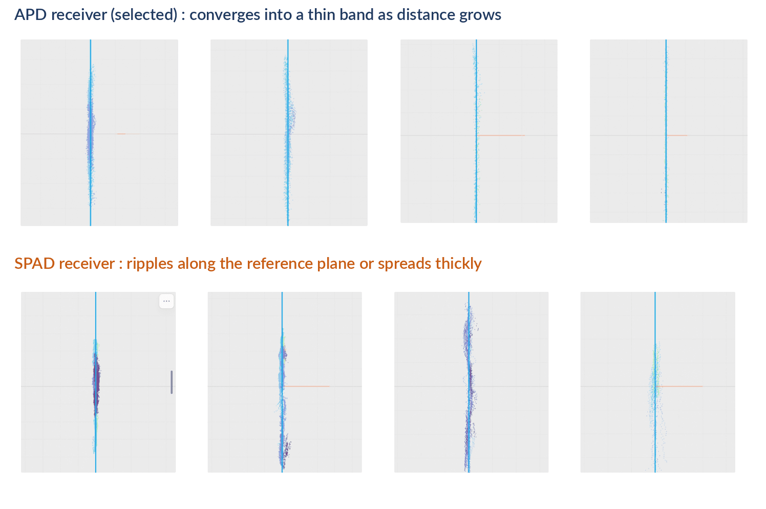
Point clouds seen edge on. The blue vertical line marks the true wall position, and the more tightly the points hug that line, the more accurate the measurement.
More Points, but Accuracy Won
Point density was the one spec that held. The SPAD receiver LiDAR returned nearly seven times as many points in the same area. On density alone, that is a clear advantage.
We chose the sparser but more accurate sensor anyway. What a robot needs inside a metal structure is not data that fills a wide area densely. It is data that tells you without wavering where the walls and floor actually are. However many points you collect, if they scatter above and below the true plane, the position estimate built on them wavers by the same margin.
The last gate was registration. We ran the point cloud from this sensor through alignment against the structure's design drawings, confirmed that it locked on consistently across access holes, stiffeners, and full wall spans, and only then designated it the primary sensor. The final criterion was never whether the sensor produced data. It was whether position estimation held up on that data.
After three swaps and field testing at three sites, the configuration we settled on is four RGB cameras and two LiDAR units. The two LiDAR units establish the reference for distance and geometry while the four cameras fill in color and texture. The cameras are arranged to face non-overlapping directions, which reduces blind spots.
Binding Many Eyes into One Frame
Changing the sensor changed the nature of the data. A depth camera outputs a 2D depth map with a distance value at every pixel, so moving that into the 3D coordinates the robot works in requires a conversion through the camera's intrinsic parameters. Whatever error those parameters carry lands directly in the result. LiDAR outputs 3D points from the start, so that conversion step disappears.
A new problem takes its place. Mounting several sensors reduces blind spots, but each one sees the world in its own coordinate frame, so the same structure appears at a different position depending on which sensor you ask. In this state the data cannot be merged into a single map, and changing sensor types does nothing to fix it. Resolving this is what calibration does.
Internal Optics and External Placement
Calibration recovers two kinds of values.
Intrinsic parameters | Extrinsic parameters | |
What it is | The camera's own optical characteristics | Where the sensor sits in space and which way it faces |
Components | Focal length, principal point, distortion coefficients | Rotation and translation |
How often | Once per unit | Every time the sensor moves |
Without it | You cannot tell which direction a pixel points | You cannot merge data from multiple sensors |
Distortion splits into two kinds: radial distortion, where lens curvature bends straight lines, and tangential distortion, which arises when the lens and sensor are not perfectly parallel.
The two parameter sets work in sequence. Extrinsics move a point in space into camera-relative coordinates, then intrinsics project that point onto pixel coordinates. You need both to recover a real 3D coordinate from a pixel and a distance value.
Why Every Shot Needs a Different Angle
The usual tool for this calculation is a checkerboard, because it is a planar pattern whose real dimensions, such as the spacing between corner points, are known in advance.
The calculation works precisely because the checkerboard is planar. The relationship between points on that plane and points in the image is expressed by a single matrix, and inside that matrix the camera's intrinsic parameters and the camera pose at capture time are multiplied together. Compute this matrix for each of several images and the pose, which differs shot to shot, disperses, leaving only the intrinsic parameters that every image shares.
How many images you need falls out of simple counting. One image supplies two constraints while there are five intrinsic parameters to solve for, so three images is the theoretical minimum. In practice, noise pushes you to shoot ten to twenty.
One condition is decisive here. The checkerboard has to be tilted to a different angle every time. Shooting many frames from the same pose only repeats the same mathematical constraint and adds no new information.
When Fields of View Do Not Overlap
For sensors whose fields of view overlap, working out the relative position between them is straightforward. They can look at the same checkerboard simultaneously. The problem arises when a robot's sensors face outward in different directions to minimize blind spots. Without overlap, they cannot see the same pattern at the same time, and the direct route to computing the relationship between them disappears.
The workarounds that exist all carry a cost. Inserting an intermediate sensor so the views chain together does connect them, but it is cumbersome and accumulates error. Building a checkerboard large enough for every sensor to see at once is impractical, and bringing in external position-measurement equipment is expensive and complex.

Turning sensors outward to reduce blind spots means their fields of view no longer overlap. With no shared view of the same pattern, there is no direct way to compute the relationship between them.
The approach DIDEN Robotics took is to fix the patterns relative to each other and use the robot itself as the link. Mount several patterns rigidly on a single structure and the relative positions between those patterns stay constant. How each sensor sees whichever pattern is in front of it can be measured, and since the sensors are fixed to the robot, moving the robot lets each sensor observe several patterns in turn. The fixed inter-pattern relationships then connect the sensors' relative positions into a single system of equations, and once you accumulate enough combinations of pose, pattern, and sensor, that system resolves. The sensors end up in one coordinate frame without ever sharing a field of view.

Pattern placement, robot motion, shared-variable linking, and global optimization. Four steps bind sensors with no overlapping view into a single coordinate frame.
The pattern here is a ChArUco board rather than a plain checkerboard. A checkerboard localizes corners to sub-pixel precision but gives no way to tell which corner is which, so the whole board has to be visible. ArUco markers carry unique IDs and can be identified from a partial view, but their corner precision is lower. A ChArUco board places ArUco markers inside the white squares of a checkerboard and gets both properties: identify position by marker ID, then localize the nearby checkerboard corners precisely. When you scatter multiple patterns and move a robot among them, you need to know which pattern you are currently looking at, and parts of the board are frequently occluded by the robot's own body, so both properties are required.
Too Little Rotation, No Solution
The first time DIDEN Robotics applied this method, it failed. The initial data collection gave the robot only yaw rotation in place. When rotational diversity is insufficient, the system of equations has no unique solution. It falls into a mathematically singular state where the calculation does not resolve at all. Only after recollecting data with the robot moving across all three rotational axes did the solution emerge, and sensors that shared no field of view were unified into a single coordinate frame.
The reason a checkerboard has to be tilted differently for every intrinsic calibration shot and the reason the robot has to be rotated across three axes here are identical. Without pose diversity, the equations only repeat the same constraint.
Calibration succeeds or fails on how the data is gathered. What poses you use, how widely you vary them, and how you secure the lighting and standoff distance that keep markers sharp are what determine the result. A minimum of ten valid images per sensor is the common recommendation, but scattering the poses matters more than hitting the count. Controlling these conditions requires being able to design the robot and drive its motion yourself.
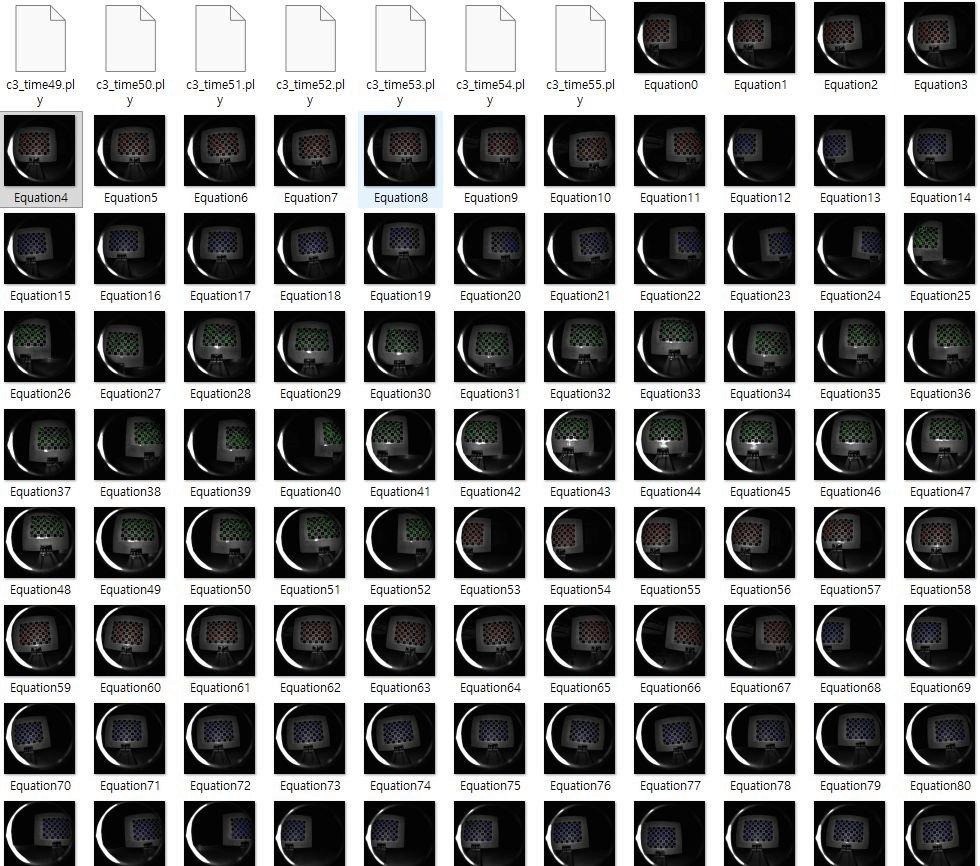
Collected data capturing the same pattern from many different poses. How widely the poses are scattered matters more than how many frames you gather.
Designing Backward from Control
Even after the sensors are chosen and the coordinate frames are bound, one question remains: in what form does this data reach control? The two preceding stages were carried out against the answer to that question. It is also why the final criterion for sensor validation was the behavior of the perception algorithms.
That ordering is only possible because DIDEN Robotics builds those algorithms in-house. The evaluation tools that judge a sensor, the calibration pipeline that binds several into one frame, the registration that aligns point clouds to design drawings, the algorithms that estimate the robot's own position and build maps on top of that, and the control and learning that take those results and decide how to move are all developed internally. Because every stage downstream could be rerun whenever a sensor changed, the criterion could sit with the algorithms rather than with the sensor.
What control asks of vision divides into four categories.
Category | What it tells you | Where it goes |
Spatial | What is where | Constraints for path planning |
Temporal | How the surroundings will change in the near future | Velocity controller, model predictive controller |
Physical | Material properties and how to handle them | Arm trajectory, gripper force |
Semantic | What the object is and what is happening now | Task success or failure judgment |
Where Each of the Four Goes
The basic unit of spatial information is the occupancy map. Space is divided into a grid, and each cell is filled with the probability of an obstacle, distinguishing what is passable, what is blocked, and what has not been observed yet. Layering distance to obstacles and surface risk onto that as a cost gives you the cost map, and the two together become the constraints for path planning. Blind spots then convert into safety margins, and collision risk is reduced at the planning stage rather than at execution.
Temporal information supplies the velocity and acceleration of approaching objects and where they will be seconds from now. This is what separates control that reacts after an obstacle moves from control that steers clear of its path in advance. Physical information is needed the moment a robot arm grasps something, because where and how firmly to grip depends on material and shape. Semantic information judges whether the task succeeded. A robot can execute the turn-and-pull motion on a door handle perfectly, but if the door did not open, the task failed, and joint angles alone cannot tell you the difference.
What Changed, and What Remains
Repeatability changed the most. In the depth-camera era, the same commanded motion put the foot down about 1 cm off from one trial to the next. For work that requires settling precisely into the narrow space between stiffeners, that variation was a real burden. With LiDAR as the primary sensor, we have confirmed repeatability at the 1 cm level over repeated trials, and the robot now lands in the same spot closely enough that the difference is hard to see by eye. It has also reached the point of recognizing and responding to a person walking past or a cable lying across the floor.
The character of the data changed as well. One hour of operation accumulates roughly 50 GB across LiDAR, cameras, joint and inertial sensors, and error logs. Build the structure that loads this onto a server and feeds it back into training, and every hour the robot spends working becomes material for the next model.
What remains is pushing precision one order finer. The current configuration secures the accuracy needed for locomotion and posture, but work like welding, which demands millimeter-level precision, is a different problem.
Here the error stacks in two layers. One is the gap between the design drawing and the structure as it was actually built. The other is the error in the registration algorithm that aligns the point cloud to that drawing. Together, they make it difficult to hold a position within 1 cm in tight spaces such as the gap between stiffeners. Ultra-precise measurement in metal environments is a limit shared by every sensor we have tested.
For that band, DIDEN Robotics is separately evaluating micrometer-class laser precision measurement sensors. This would not replace the current configuration but add to it, giving the robot one set of eyes for moving and another for working.
What Comes After the Sensor
For a robot on an industrial site, perception is raw material for a decision. It exists to determine where to step, what to grasp, and whether the last action actually worked. It is not an end in itself. Building a perception system is therefore not a matter of comparing parts. It starts from the judgments control has to make, defines the outputs those judgments require, and works backward to a configuration capable of producing them.
This is the same way DIDEN Robotics has approached actuators and learning. Rather than finishing the hardware first and layering software on afterward, both sides define what they require of each other and are designed together. It is why hardware constraints set the first sensor and hardware later changed in response to what perception demanded, and why four rounds of validation were needed to settle the configuration. At every stage, the criterion was not the sensor's own performance but the behavior of the algorithms running on top of it.
[How a robot finds itself and reconstructs its surroundings in 3D] was covered in an earlier post on this blog. This one steps back one stage further, to what kind of data sits at the place where all of those calculations begin. That is why DIDEN Robotics, a physical AI company for industrial environments, validates a robot's eyes starting at the sensor.
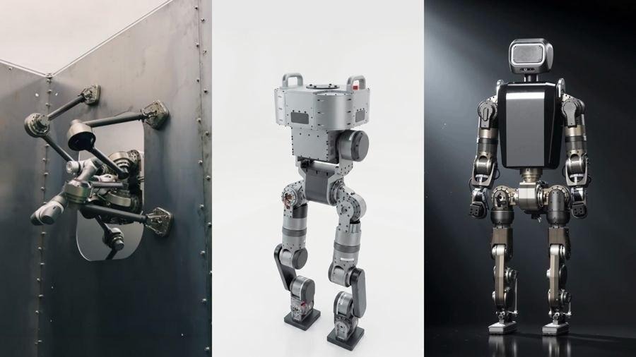
At DIDEN Robotics, perception, control, and learning are designed together inside one team.
More from Diden Robotics

The Five Branches of Diden Robotics' Control Electronics: Circuit Design Started with In-House Actuators and Magnetic Feet
Blog
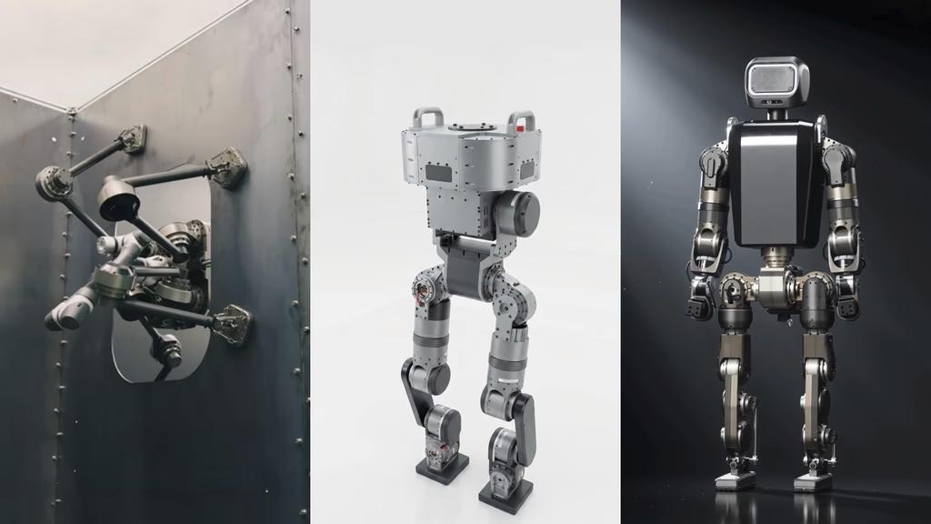
Why a Quadruped, a Biped, and a Humanoid All Walk the Same Way: Co-Designing Actuators and Learning
Blog
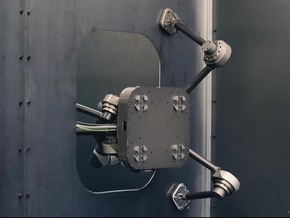
How a Robot Makes Moves No Human Has Ever Shown It
Blog
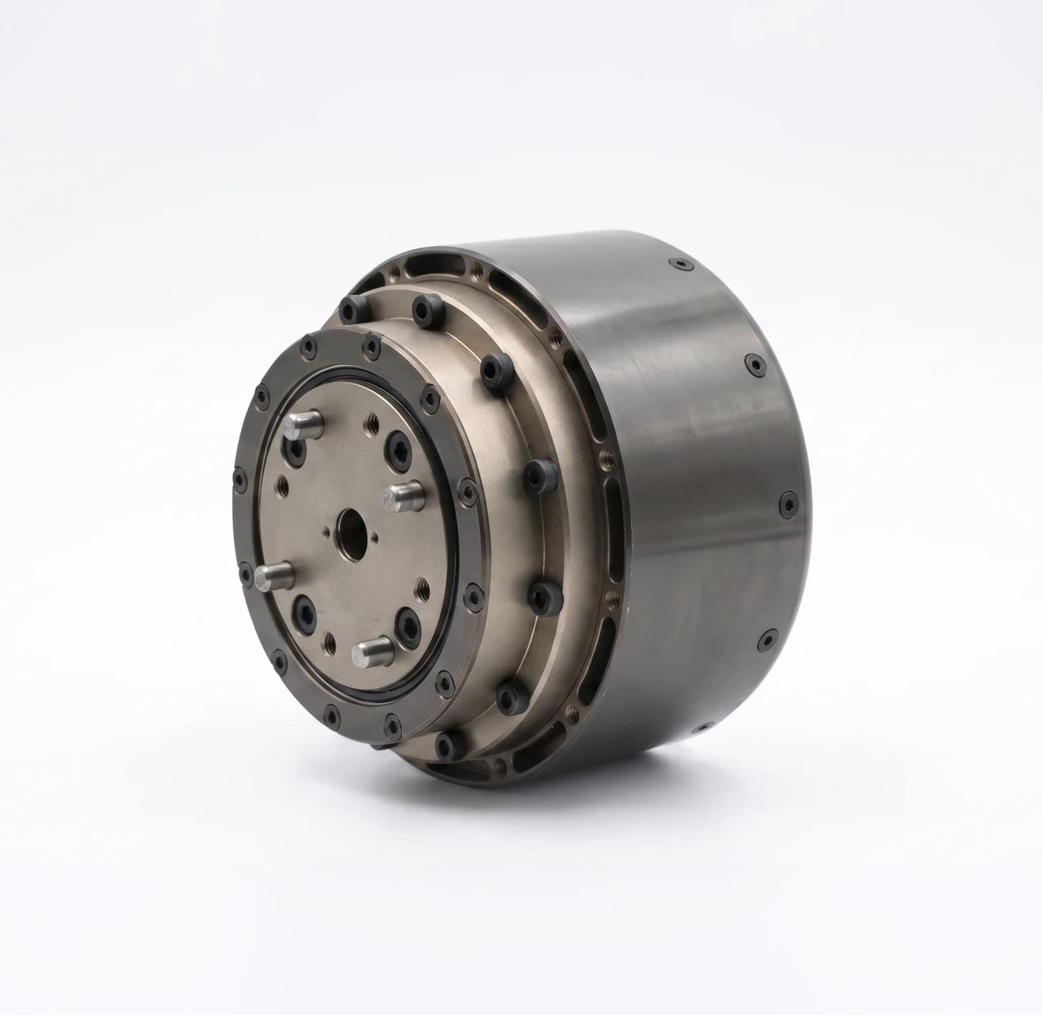
Why DIDEN Robotics Builds Its Actuators In-House
Blog